AN INSIGHT INTO THE FUNDAMENTAL PHYSICS OF ENGINE PERFORMANCE
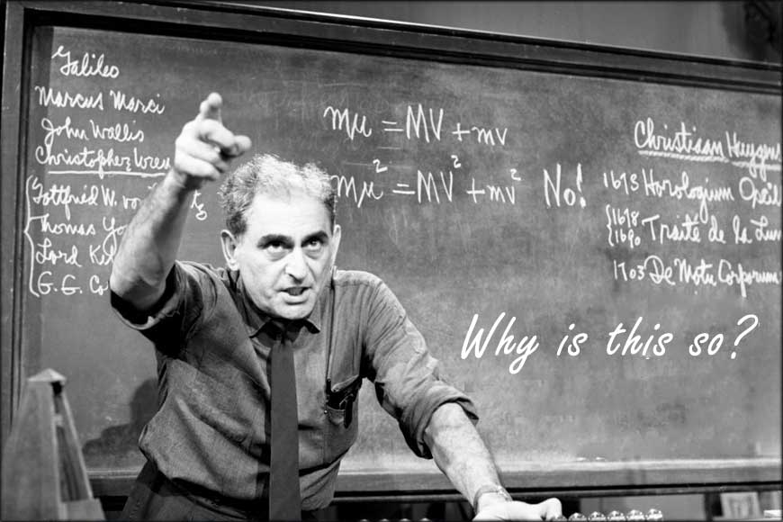
WHY IS THIS SO?
To the readers who are experts in engine design theory this article could be ‘old hat’ so I apologize for boring them and wasting their time.
To others perhaps less theoretically agile, this should be welcome as it will compare design concepts with numbers rather than argument.
We hope you enjoy the following information to better understand the math myths behind engine improvements and how RACEHEAD ENGINEERING improves performance.
The Basics
An engine is a device with a number of cylinders each with a cylinder bore (B) and a stroke (S). This gives the engine a swept volume (Vsv) for each cylinder and a swept volume for the entire engine (Vtsv). The engine will have a bore to stroke ratio (Kbs). The calculation of this basic data is shown in equations 1-4.
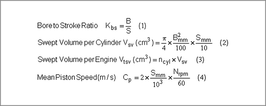
A further important mechanical design parameter is the mean piston speed (Cp), For racing engines, this limit parameter has hardly increased in numeric value in fifty years and that fact reflects the gradual improvement of cylinder design and lubrication technology since the 1950s.
Then, an air-cooled and iron linered Norton Manx cylinder had a mean piston speed of 20 m/s at its engine speed for peak power. Today, a MotoGP engine at peak power with its liquid-cooled and silicon-carbide plated cylinder running on a synthetic lube oil has a mean piston speed of 25m/s. One would be hard put to call that a technological breakthrough.
“Racing engine mean piston speed has hardly increased in numeric value in fifty years”
THE FUNDAMENTALS
A firing engine produces a turning moment at the crankshaft, the TORQUE. Depending on the speed of rotation of the crankshaft (N) the engine produces a power output (POWER). The TORQUE is measured with the engine on a dynamometer.
The computation of the POWER output is shown in equations 5-8 There the unit is POWERkW (kW or kilowatts) but if you want horsepower (bhp) instead then divide POWERkw by 0.7457 to get POWERbhp.
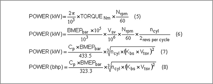
Alternatively, one can compute the POWER using the brake mean effective pressure (BMEP). However, and much more likely, having used the measured TORQUE to get the power output from the dynamometer data, you can calculate the value of the BMEP by back-calculation using a re-arranged Eqn.6, because all other parameters are known data values for the engine.
Somewhat like mean piston speed, this is another parameter which, for the naturally aspirated, gasoline racing engine, has barely changed over the last fifty years. That Norton Manx racing motorcycle of 1955 attained a BMEP value of almost 14 bar.
Today’s MotoGP engine also has a BMEP value of about 14 bar. Some progress! However, that 800 cc MotoGP engine does it at 17,000 rpm whereas the 500 Norton did at 7000 rpm so the power differential is huge. As the BMEP potential and the piston speed are such common parameters between engines, the Eqns.7 and 8 become very useful ready-reckoners as to the possible power performance of any engine.
The highest mean piston speed (Cp) I have heard of at the time of writing this article is 26.5 m/s but these boundaries are increasing continually with the development of high strength lightweight materials so in particular the RPM of large displacement drag race engines increases every year! However the maximum BMEP potential of the simple naturally aspirated, gasoline four-stroke racing engine at high piston speed is some 15 bar, this limit has not changed much at all.
Nevertheless, Eqns.7 and 8 still permit you to make quick design decisions as to what performance is potentially possible from any engine. It also permits you to numerically trip up those PR-based engine developers who grossly exaggerate their engine’s power output as evidence of the application of their genius!
“Those engine developers who grossly exaggerate their engine’s power as evidence of their genius!”
THE MEAN EFFECTIVE PRESSURE
Ok so far we have covered some basic principles of engine physics from now on it gets a little more complicated.
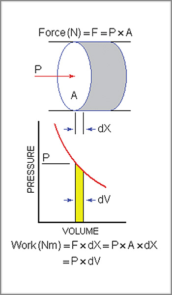
Work is defined as the distance (dX) moved by a force (F). In the context of a piston in a cylinder, as seen in Fig.3, the force (F) on the piston is the product of the pressure (P) on it when applied over the piston area (A).
Hence, the work done on, or by, the piston as it moves is the product of the pressure (P) and the cylinder volume change (dV) as it occurs.
On the power stroke, as the volume increases that work is positive.
On the compression stroke, as the volume decreases that work is negative, i.e., supplied by the engine to the piston.
During the power phase, from bottom dead centre (bdc) to the next bottom dead centre (bdc), or one turn of the crankshaft, the pressure-volume diagram of the in-cylinder events is shown in Fig.4.
It is sketched from data for the MotoGP engine. The net work (POWER WORK) on the piston during this process is the summation (integration) of all of the pressure volume increments over the period and is shown as the area coloured yellow in the diagram.
If there were no other losses in the system, that would be the work delivered to the crankshaft; but there are.
The yellow area can be represented by the equivalent rectangular area shown in blue, which area has a height of IMEP and a width of the cylinder swept volume (Vsv).
The value of IMEP is known at the indicated mean effective pressure. It is called ‘indicated’ as it is derived from the pressure transducer signal as measured in the cylinder head of the engine.
During the pumping phase that follows, from bottom dead centre (bdc) to the next bottom dead centre (bdc), or the next turn of the crankshaft, the pressure volume diagram is shown at the right of Fig.4.
Here, the work computation would elicit a negative value for the PUMP WORK, the yellow area on that diagram, as the opening (higher) line is of compression (negative dV) during the exhaust stroke.
This yellow area can be equally represented by the equivalent rectangle of height PMEP and width Vsv labelled as the pumping mean effective pressure. Its negative numerical value indicates that the pumping work is supplied by the piston from the crankshaft; in short, it is lost work.
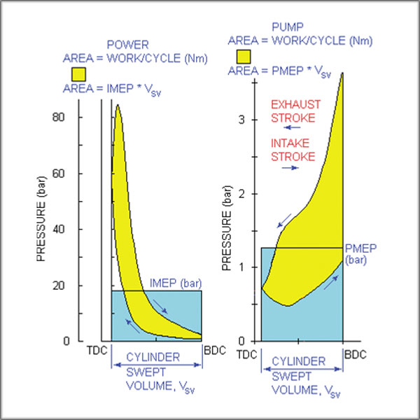
The rest of the engine work losses are lumped together as ‘frictional’ losses and can be expressed as a FMEP value, the friction mean effective pressure, again officially a negative number. The upshot of this part of the discussion can be seen in Eqns.9-14.
The net work per cylinder per cycle is shown in Eqn.9 where the brake mean effective pressure (BMEP) is observed to be the result of subtracting the (positive values of) the pumping mean effective pressure (PMEP) and the friction mean effective pressure (FMEP) from the indicated mean effective
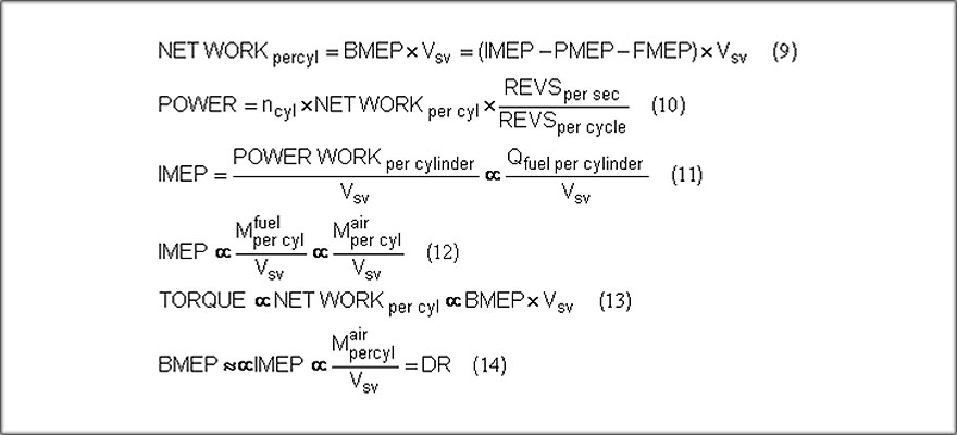
pressure (IMEP). AS IMEP and PMEP data can only be determined from an analysis of measured cylinder pressure diagrams, but BMEP can be calculated from measured dynamometer data through Eqns.6-7, then one method of determining FMEP is through the re-arrangement of Eqn.9.
The ratio of BMEP to IMEP is known as the ‘mechanical efficiency’ of the engine and is normally in the 75 to 85% range for most racing engines. The MotoGP engine [2], designed for a BMEP of 14 bar at 16,100 rpm, produced exactly that. It had a IMEP value of 18.52 bar, a PMEP value of 1.26 bar (see Fig.4) and a FMEP value of 3.26 bar; the mechanical efficiency was 75.6%.
THE CONNECTION BETWEEN MEAN EFFECTIVE PRESSURE AND AIRFLOW
In Fig.5, Eqn.11, it can be seen that IMEP is the POWER WORK divided by the cylinder swept volume. Alternatively, that in-cylinder work is directly proportional to the heat released (Q) by combustion of the fuel trapped in the cylinder.
In Eqn.12, this argument is advanced to relate the heat released (Q) to the mass (M) of fuel trapped in the cylinder. However, as air-fuel ratios for racing engines on gasoline are almost fixed, Eqn.12 reduces to showing that IMEP is directly proportional to the mass of air (Mair) trapped in the cylinder.
It is but a short logical step in Eqn.14 to relate the BMEP to IMEP and the BMEP to the specific mass airflow rate into the engine, i.e., delivery ratio (DR). An even shorter logical step is found by linking Eqns. 13 and 14 to relate the engine TORQUE output per cylinder to BMEP and DR.
“The MotoGP engine designed for a BMEP of 14 bar at 16,100rpm had a mechanical efficiency of 75.6%”
In short, as BMEP and DR have only minor variations from one racing engine to another, BMEP and DR are far more useful numbers with which to compare the development level of differing engines than is the output TORQUE, because this number also incorporates the total swept volume of an engine.
The bottom line, design-wise, is that brake mean effective pressure (BMEP) is inextricably linked with the specific mass airflow rate ratio, delivery ratio (DR).
In this discussion, you will note that I have not used or defined the term ‘volumetric efficiency’, which is a volume based specific airflow rate parameter ignoring air mass/volume variations such temperature, atmospheric and altitude conditions.
THE ONWARD CONNECTION BETWEEN AIRFLOW AND DESIGN
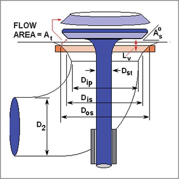
An engine inhales air through its intake valve(s) and exhales through its exhaust valve(s). The aperture area (At) through which this flow takes place at any valve lift (Lv) is shown in Fig.6.
Also shown is the basic geometry of a valve seat, a valve seat angle, a valve stem, an inner port, and a duct size at the manifold.
The physical dimensions are labelled as the valve seat angle (As), the diameters at the seat (Dis and Dos) and at the inner port (Dip), and at the manifold (D2).
The manifold diameter (D2) may connect to a number of valves (nv) so, if so, the total aperture area for flow is obviously a multiple (nv times At) of that illustrated for one valve.
The aperture flow area (At) is considered as being the side area of a frustum of a cone and that cone shape changes position with lift.Iif all analyses are to be accurate,
it must be persistently used to the point of pedantry in absolutely every aspect of the design process from the experimental determination of discharge coefficients (Cd), valve flow time-areas, through to implementation within a theoretical engine simulation. The theoretical computation of the airflow rate is conducted through complex equations.
“It must be persistently used to the point of pedantry in absolutely every aspect of the race engine
design process”
At any one step, the effective area of the aperture is the product of the discharge mass flow coefficient (Cd) and the area (At).
The volume flow is found by multiplying that value by the particle velocity, and the mass flow rate by multiplying that product by the prevailing gas density (rho).
The summation is conducted over the main part of the intake stroke from tdc to bdc. This is the complex step by step integration that proceeds incrementally.
However, this computational approach for the delivery ratio (DR),will never be executed on your pocket calculator

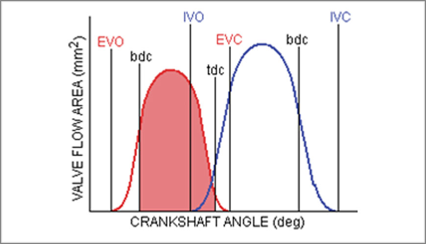
The main variables vary dramatically during the summation process from tdc to bdc. Above shows the variation of the particle velocity (c) at the manifold diameter (D2) for both the exhaust and the intake processes; the value is plotted as Mach number which is particle velocity (c) divided by the local acoustic velocity.
For the intake flow, from tdc to bdc, the particle velocity rises from near zero to a Mach number of about 0.5 However, while these variations are significant and would inhibit the ‘pocket calculator’ solution for DR the pattern of all these variations from engine to engine is really quite similar.
Hence, citing these similarities, we can solve for what is known as the specific time area (STA) shown by the graphical result
it is the area coloured blue in the diagram which is the integration of the intake aperture area from tdc to bdc.
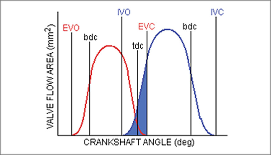
The entire intake valve period extends from opening (IVO) to closing (IVC), but the STAip data refers only to the main intake pumping period from tdc to bdc.

The result of the equivalent calculation for the exhaust pumping period, the exhaust stroke from bdc to tdc for the exhaust valve and is labelled as STAep.
By definition, any air mass induced into the engine inevitably becomes the exhaust mass post-combustion (plus the added fuel mass) and which requires to be expelled from the engine.
Therefore, there is an obvious proportionality connection between the STAip and STAep values.
In a racing engine with tuned intake and exhaust systems, scavenging of the trapped exhaust gas during the valve overlap period from the small space that is the clearance volume is a vital part of effective engine design.
This permits a through-draught of fresh charge to scavenge the cylinder of its exhaust gas and fill it with fresh charge.
If carried out effectively say, in an engine with a compression ratio of 11, it means that the induction process can begin with a delivery ratio of some 10% before the downward piston motion even begins to suck in air, 10% extra DR can be 10% extra BMEP.
The scavenge process will only be successful, always assuming that the intake and exhaust tuning is well organized, if the phasing of the opening intake valve and the closing exhaust valve apertures is effective.
This phasing is well-expressed pictorially by the specific time areas for the overlap valve periods for the exhaust valve(s) (STAeo) and the intake valve(s) (STAio) as the red and blue coloured areas, respectively.
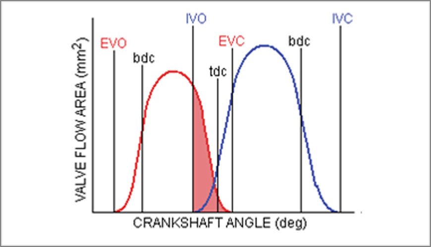
If either value, or both, is numerically deficient then, even with perfect pressure wave tuning, the throughflow scavenge process will be impaired, as will the engine POWER.
In a two-door room with both doors shut, there are no draughts on a windy day.
Another valve area segment to be considered is the period from the opening of the exhaust valve(s) to the bdc position, i.e., the exhaust blowdown period. The specific time area for this period (STAeb) is shown, coloured red
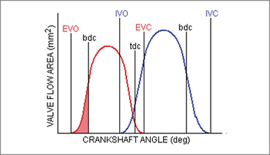
If this value is numerically inadequate then the cylinder pressure at bdc will be high as a sufficient mass of exhaust gas has not been bled from the cylinder. Hence, the ensuing exhaust pumping process from bdc to tdc will be conducted with higher than normal cylinder pressures giving increased pumping losses (PMEP) and may even promote excessive exhaust gas backflow up the intake tract as the intake valve opens.
If this latter situation occurs, even a well-designed scavenge process could be negated because it would be conducted with backflow exhaust gas and not fresh intake charge; a situation guaranteed to invisibly and inexplicably reduce power output, raise the trapped charge temperature and encourage detonation.
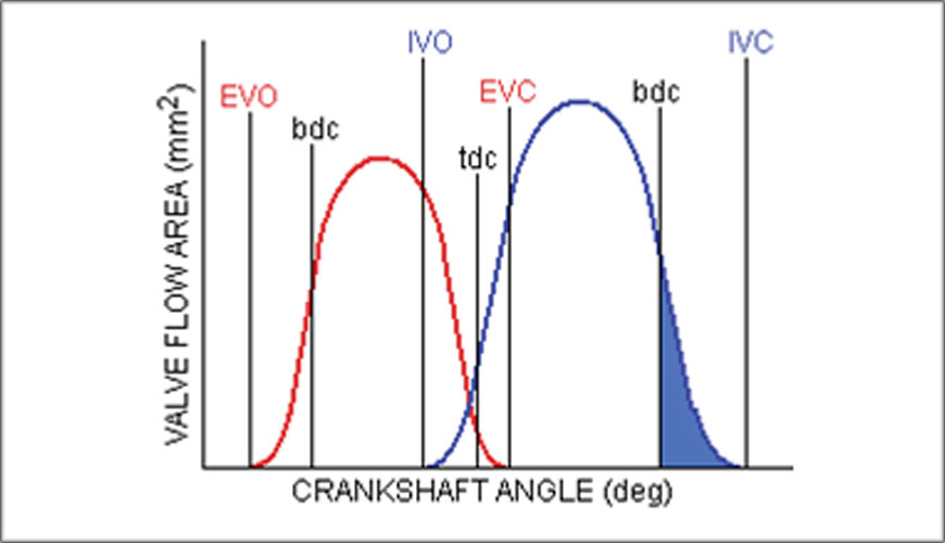
The final valve area segment to be considered is the period from the bdc position on the intake stroke to intake valve closure at IVC, i.e., the intake ramming period. The specific time
area for this period (STAir) is shown, coloured blue.
The higher is the desired delivery ratio (DR), the higher required BMEP, then so too must be the need for effective intake ramming which requires sufficient valve aperture and time at any engine speed.
That a well-designed and phased intake system will give the correct direction of pressure differential to encourage a ramming action can be observed from bdc to IVC.
THE CONNECTION BETWEEN SPECIFIC TIME AREA AND DESIGN
Many engines, ranging from high performance racing engines to lawnmowers, all at their engine speed for peak horsepower, have indeed a logical numerical connection between their individual STA values and the BMEP attained by them.
There was, naturally, scatter in this plethora of data from so many sources, but the trends were very clear. A theoretical connection between STA and BMEPcan be established and reduced to equations and one can match the six individual STA values as closely as possible to their target values for a required BMEP.
What is important is not to have any one STA value seriously deficient of its target value as that will make the design ‘unmatched’ and the engine will breathe badly.
Although the equations can be solved on your pocket calculator, it is too complicated to produce the actual STA values for a given engine. This requires the numerical integration of the six segments of the two valve lift curves and their aperture areas.
Today, the likes of 4stHEAD software the STA analysis for the empirical design of a new engine, or analysis of an existing one, is conducted within a dedicated computer program. In such software, the STA-BMEP equations have been enhanced and extended to cope with both spark-ignition and compression-ignition engines; with the use of gasoline, kerosene, methanol and ethanol fuels; with the employment of differing compression ratios; and the use of supercharging or turbocharging.
THE CONNECTION BETWEEN THE VALVE APERTURES AND THE DUCTS
The high cylinder pressure during exhaust blowdown, and the low cylinder pressure during the induction stroke, creates compression waves and expansion (suction) waves in their respective ducts. It is the reflection of these waves at the exhaust pipe end (or mid-section expansions at a branch or collector), or at the bellmouth of the intake, which provides the pressure differential characteristics to conduct cylinder scavenging during the exhaust overlap period. In the case of the intake, that tuning length also needs to be set correctly to aid the ramming process.
Apart from designing in the correct lengths, the size of the ducts at the manifold is a most important design consideration and one which is rarely, if ever, emphasized in published empirical theory.
If the ducts are too large then the pressure waves will be weak except at the very highest speeds and if too small they will yield waves of excessive amplitude except at the lower engine speeds.
Upon pipe end reflection, weak waves give less effective pressure differentials for the scavenge or ramming processes and waves of excessive amplitude friction-scrub themselves along the pipe walls with an inevitable reduction in their strength giving the same outcome.
Analysis of many engines, both empirically from their physical geometry and theoretically using complete engine simulations, yields empirical design criteria for the optimum size of these ducts. The empirical criteria relate the manifold duct size to their valve apertures and the number of valves providing them.
DESIGN USING EMPIRICAL CRITERIA
The specific time areas (STA) are incorporated into a design for a piston speed (Cp) of 25 m/s and a BMEP of 14 bar with the exhaust and intake duct sizes. It’s not possible to meet all STA target values precisely, nor is it vital as empiricism is not an exact science! The reason one cannot precisely mesh actual and target STA values is that one must work within the confines of real valve lift profiles that must also survive without failure.
This data can be presented to an accurate engine simulation and run over a specified speed range with differing sizes of exhaust and intake ducts. The results for POWER and airflow rate (DR) rate can be noted. The largest duct pairing gives the highest power and airflow at the higher engine speeds but loses out at lower rpm.
However, the larger duct pairing may exceed the designed power output of (14 bar BMEP at given rpm) So at the expense of a ‘peaky’ power curve and an even ‘peakier’ airflow curve; the latter may not provide the actual power estimated in the real world and provide on-track difficulties in fuelling smoothly.
The duct sizes should match the design power criterion exactly. The applied Km criteria reveal that the duct size variations from the designed value by about +/- 1 mm for ‘acceptability’ and that ‘acceptability’ is well-nigh proven as these Km criteria exhibit a very narrow dimensional tolerance.
This evidence should provide a cautionary tale for those who may somewhat arbitrarily size their engine ducts and are even now pondering the reasons behind either ‘peaky’ power curves or ‘inadequate’ peak power curves when, by their design lights, they ought to have been ‘perfect’. In short, a well-executed design using the STA-BMEP parameters can be negated to some extent by an incorrect sizing of the intake and the exhaust ducting.
“A well-executed design can be negated to some extent by an incorrect sizing of the intake and the exhaust ducting”
I regret to say that, while this is a design criterion for the dimensions of an intake valve and is doubtless helpful in that regard, further assistance is not forthcoming for the rest of an engine design.
However, if one replaces the mean piston speed with the maximum piston speed (Cp) in Eqn.26, i.e., the above-used number 25 would virtually double to about 50 m/s, the Mean Gas Velocities then double to 168.8 and 152 m/s, respectively, the first of which is not a million miles/hour away from the Mach number optimum of 0.5 (170 m/s) debated above.
This reasonable correlation, between Mach number and a Kl value based on maximum piston speed, lends theoretical credence to its usefulness as a basic method to size an intake valve.
Moreover, if one extends Mean Gas Velocity thinking to the exhaust valves of an engine, where the speed of sound in the elevated temperatures of exhaust gas is some 600 m/s, there the Mach number criterion of 0.5 translates to (if computed at maximum piston speed) a Mean Gas Velocity of 300 m/s. For the exemplar MotoGP engine, using 50 m/s as the maximum piston speed and 22 mm which is the inner port diameter (Dip) of each exhaust valve, the exhaust valves area ratio (Kev) is 0.177 from Eqn.25, and an exhaust-based Mean Gas Velocity becomes 284 m/s from Eqn.26; and that is a pretty good match for the supposedly required value of 300 m/s. Hence, it seems feasible to extend the Mean Gas Velocity concept to the exhaust valves as well; this is important as the relative sizing of the exhaust and intake valves is a critical design factor which has been previously discussed.
However, while the basic sizing of the valves in any given design may well be guided by using the Mean Gas Velocity for the intake valve(s) and also by this extension for the exhaust valve(s), it falls short of telling us what to do with either of them to tailor a required engine power characteristic.
Firstly, there is no information as to the valve lift profile which should accompany a Mean Gas Velocity; such as how high should the valve(s) be lifted?; such as the required duration or the angular positions of valve opening or closing or maximum lift?; or what happens if I employ a more or a less aggressive valve lift profile?
Secondly, in the absence of an extension of the Mean Gas Velocity concept to dimension the exhaust valves, we would not know the required size of the exhaust valve(s) which should accompany the intake valve(s); or how high and for how long, and when, they should operate, etc., etc?
The good thing about the Mean Gas Velocity (Kl) concept is that it can be easily derived on a hand calculator but as a design tool, even with the above-proposed extension for sizing exhaust valves, it is much too simplistic to be universally useful.
Technical journalists et al should consider quoting Kl data with the relevant caveats and not as Holy Grail. It was, as I understand it, the late Brian Lovell of Weslake who conceived Mean Gas Velocity with respect to intake valves.
Before I get literally savaged by some technical journalist who feels that I have demeaned the memory of a great design engineer, I should point out that Brian Lovell proposed Mean Gas Velocity as a means of comparing engines for which precious little data was available in a design era populated with slide rules and not computers; more complex calculations were definitely not on the menu.
CONCLUSIONS
If I have thoroughly bored my expert reader I can only but repeat my earlier apology; the fault is yours, you should have stopped reading back at the first page!
To those to whom this paper is a refresher course from their university days, then that is no bad thing. Although I very much doubt that your undergraduate university course ever extended to unsteady gas dynamics, pressure waves and engine tuning, not to speak of specific time areas, to be reminded of the fundamentals and see them extended into effective design techniques is, as has been said before, no bad thing.
To those who find even this level of math somewhat daunting, but yet have a basic understanding of engine tuning, rest easy because all the mathematics of unsteady gas dynamics, valve lift profile design, valvetrain dynamic analysis, cylinder pressure analysis, discharge coefficient analysis, and specific time area calculations are packaged nowadays into computer software that you can effectively use for design and thereby gain total understanding of the theoretical concepts which are discussed here.
Why is this empiricism so important if all I have to do is buy a complete engine simulation, like I use here, and just keep stuffing the input data numbers of the engine and duct geometry into it until I come up with the required engine design?
This is especially the question as some of these engine simulations come with built-in automatic performance optimisers [7].
The answer is that you can keep stuffing numbers as input data into an engine simulation, where the data involved number in the hundreds if not thousands, but you may never attain a design as well optimised as the exemplar MotoGP engine [2].
The reason is that it was initially created in the 4stHEAD software using the above empiricism to reach a ‘matched’ design which employed real valve lift profiles that not only provided valvetrain dynamic stability but also a satisfactory cam design and manufacture potential.
It was only when all such design considerations were satisfied that it was run through the engine simulation to check that, as shown in Fig.21, (a) the design target was achieved and, (b) an effective power and torque characteristic extended over the usable speed range.
All readers, be they experts or tyros, must conclude that does constitute a design process. In short, it is through an understanding of the basics that we get the guidance to efficiently use today’s sophisticated computational tools for engine design.
REFERENCES
[1]G.P. Blair, sidebar contribution on combustion in diesel engines, Race Engine Technology, Volume 5, Issue 2, May2007 [2]G.P. Blair, “Steel Coils versus Gas”, Race Engine Technology, Volume 5, Issue 3, June/July 2007 [3]G.P. Blair, “Design and Simulation of Four-Stroke Engines”, Society of Automotive Engineers, 1998, SAE reference
R-186. [4]G.P. Blair, “Design and Simulation of Two-Stroke Engines”, Society of Automotive Engineers, 1996, SAE reference
R-161. [5]4stHEAD design software, Prof. Blair and Associates, Belfast, Northern Ireland [6]G.P. Blair, W.M. Cahoon, “Life at the Limit”, Race Engine Technology, Volume 1, Issue 004, Spring 2004. [7]Virtual 4-Stroke engine simulation, Optimum Power Technology,